Hypothesis Testing ANOVA

In the previous article, we talked about hypothesis testing using the Welch’s t-test on two independent samples of data. So what happens if we want know the statiscal significance for $k$ groups of data?

This is where the analysis of variance technique, or ANOVA is useful.

ANOVA Assumptions

We’ll be looking at SAT scores for five different districts in New York City. Specifically, we’ll be using “scores.csv” from Kaggle. First let’s get the assumptions out of the way:

• The dependent variable (SAT scores) should be continuous.
• The independent variables (districts) should be two or more categorical groups.
• There must be different participants in each group with no participant being in more than one group. In our case, each school cannot be in more than one district.
• The dependent variable should be approximately normally distributed for each category.
• Variances of each group are approximately equal.

Data Exploration

Let’s begin by taking a look at what our data looks like.

import pandas as pd 
import numpy as np
import matplotlib.pyplot as plt
import seaborn as sns
from scipy import stats
%matplotlib inline

data = pd.read_csv("scores.csv")
data.head()

	School ID	School Name	Borough	Building Code	Street Address	City	State	Zip Code	Latitude	Longitude	...	End Time	Student Enrollment	Percent White	Percent Black	Percent Hispanic	Percent Asian	Average Score (SAT Math)	Average Score (SAT Reading)	Average Score (SAT Writing)	Percent Tested
0	02M260	Clinton School Writers and Artists	Manhattan	M933	425 West 33rd Street	Manhattan	NY	10001	40.75321	-73.99786	...	NaN	NaN	NaN	NaN	NaN	NaN	NaN	NaN	NaN	NaN
1	06M211	Inwood Early College for Health and Informatio...	Manhattan	M052	650 Academy Street	Manhattan	NY	10002	40.86605	-73.92486	...	3:00 PM	87.0	3.4%	21.8%	67.8%	4.6%	NaN	NaN	NaN	NaN
2	01M539	New Explorations into Science, Technology and ...	Manhattan	M022	111 Columbia Street	Manhattan	NY	10002	40.71873	-73.97943	...	4:00 PM	1735.0	28.6%	13.3%	18.0%	38.5%	657.0	601.0	601.0	91.0%
3	02M294	Essex Street Academy	Manhattan	M445	350 Grand Street	Manhattan	NY	10002	40.71687	-73.98953	...	2:45 PM	358.0	11.7%	38.5%	41.3%	5.9%	395.0	411.0	387.0	78.9%
4	02M308	Lower Manhattan Arts Academy	Manhattan	M445	350 Grand Street	Manhattan	NY	10002	40.71687	-73.98953	...	3:00 PM	383.0	3.1%	28.2%	56.9%	8.6%	418.0	428.0	415.0	65.1%

5 rows × 22 columns

data['Borough'].value_counts()

Brooklyn         121
Bronx            118
Manhattan        106
Queens            80
Staten Island     10
Name: Borough, dtype: int64

Creating New Columns

There is no total score column, so we’ll have to create it. In addition, we’ll have to find the mean score of the each district across all schools.

data['total_score'] = data['Average Score (SAT Reading)'] +  \
                      data['Average Score (SAT Math)']    +  \
                      data['Average Score (SAT Writing)']
data = data[['Borough', 'total_score']].dropna()        
x = ['Brooklyn', 'Bronx', 'Manhattan', 'Queens', 'Staten Island']
district_dict = {}

#Assigns each test score series to a dictionary key
for district in x:
    district_dict[district] = data[data['Borough'] == district]['total_score']


y = []
yerror = []
#Assigns the mean score and 95% confidence limit to each district
for district in x:
    y.append(district_dict[district].mean())
    yerror.append(1.96*district_dict[district].std()/np.sqrt(district_dict[district].shape[0]))    
    print(district + '_std : {}'.format(district_dict[district].std()))
    
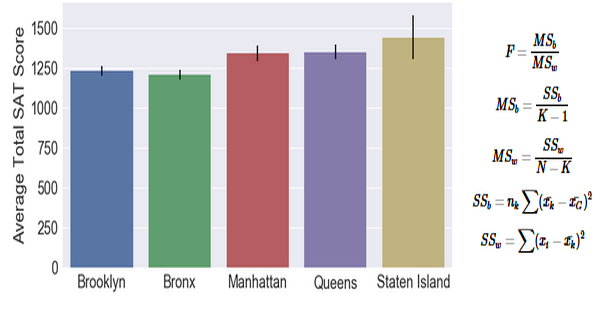
sns.set(font_scale=1.8)
fig = plt.figure(figsize=(10,5))
ax = sns.barplot(x, y, yerr=yerror)
ax.set_ylabel('Average Total SAT Score')
plt.show()

Brooklyn_std : 154.8684270520867
Bronx_std : 150.39390071890665
Manhattan_std : 230.29413953637814
Queens_std : 195.25289850192115
Staten Island_std : 222.30359621222706

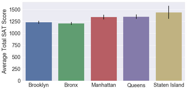
From our data exploration, we can see that the average SAT scores are quite different for each district. We are interested in knowing if this is caused by random variation in data, or if there is an underlying cause. Since we have five different groups, we cannot use the t-test. Also note that the standard deviation of each group are also very different, so we’ve violated one of our assumpions. However, we are going to use the 1-way ANOVA test anyway just to understand the concepts.

The Null and Alternative Hypothesis

There are no significant differences between the groups’ mean SAT scores.

$ H_0 : \mu_1 = \mu_2 = \mu_3 = \mu_4 = \mu_5 $

There is a significant difference between the groups’ mean SAT scores.

$ H_a : \mu_i \ne \mu_j $

Where $\mu_i$ and $\mu_j$ can be the mean of any group. If there is at least one group with a significant difference with another group, the null hypothesis will be rejected.

1-way ANOVA

Similar to the t-test, we can calculate a score for the ANOVA. Then we can look up the score in the F-distribution and obtain a p-value.

The F-statistic is defined as follows:

\[F = \frac{MS_{b}} {MS_w}\] \[MS_{b} = \frac{SS_{b}} {K-1}\] \[MS_{w} = \frac{SS_{w}} {N-K}\] \[SS_{b} = {n_k\sum(\bar{x_{k}}-\bar{x_{G}})^2}\] \[SS_{w} = \sum(x_{i}-\bar{x_{k}})^2\]

Where $MS_{b}$ is the estimated variance between groups and $MS_{w}$ is the estimated variance within groups, $\bar{x_{k}}$ is the mean within each group, $n_k$ is the sample size for each group, ${x_i}$ is the individual data point, and $\bar{x_{G}}$ is the total mean.

This is quite a lot of math, fortunately scipy has a function that plugs in all the values for us. The documentation for calculating 1-way ANOVA using scipy is here.

stats.f_oneway(
             district_dict['Brooklyn'], district_dict['Bronx'], \
             district_dict['Manhattan'], district_dict['Queens'], \
             district_dict['Staten Island']
)

F_onewayResult(statistic=12.733085029201668, pvalue=1.0161974965566023e-09)

The resulting pvalue was less than 0.05. We can reject the null hypothesis and conclude that there is a significant difference between the SAT scores for each district. Even though we’ve obtained a very low p-value, we cannot make any assumptions about the magnitude of the effect. Also scipy does not calculate $SS_b$ and $SS_w$, so it is probably better to write our own code.

districts = ['Brooklyn', 'Bronx', 'Manhattan', 'Queens', 'Staten Island']

ss_b = 0
for d in districts:
    ss_b += district_dict[d].shape[0] * \
            np.sum((district_dict[d].mean() - data['total_score'].mean())**2)

ss_w = 0
for d in districts:
    ss_w += np.sum((district_dict[d] - district_dict[d].mean())**2)

msb = ss_b/4
msw = ss_w/(len(data)-5)
f=msb/msw
print('F_statistic: {}'.format(f))

F_statistic: 12.733085029201687

To find out which specific districts differ (e.g., is Manhattan’s mean score significantly different from the Bronx’s?), you need to perform post-hoc tests, such as Tukey’s Honestly Significant Difference (HSD) test. However, this is outside the scope of this article.

The Effect Size

We can calculate the magnitude of the effect to determine how large the difference is. One of the measures we can use is Eta-squared.

\[\eta^2 = \frac{SS_{b}} {SS_{total}}\] \[SS_{b} = {n_k\sum(\bar{x_{k}}-\bar{x_{G}})^2}\] \[SS_{total} = \sum(x_{i}-\bar{x_{G}})^2\]

ss_t = np.sum((data['total_score']-data['total_score'].mean())**2)        
eta_squared = ss_b/ss_t
print('eta_squared: {}'.format(eta_squared))

eta_squared: 0.12099887621529214

The general rules of thumb given by Cohen and Miles & Shevlin (2001) for analyzing eta-squared, $\eta^2$:

• Small effect: $ 0.01 $
• Medium ffect: $ 0.06 $
• Large effect: $ 0.14 $

From our calculations, the effect size for this ANOVA test would be “Medium”. For a full write up on effect sizes click here.